Introduction to Evidential Deep Learning

– Socrates
In standard classification tasks, we have all accustomed to treating the network’s normalized probability vector as a proxy for confidence, despite its well-known limitations under uncertainty and distribution shift. In this classic setting, when the network is confident that an instance belongs to a particular class, the network assigns a high output to that class:
$$ {\mathbf{p}} = [0.9, 0.06, 0.04] $$
The network is forced to assign at least some confidence value to each class, and the confidence “mass” is spread across the class distribution. We have all treated this as the expected behavior of a deep neural network.
However, let us consider the following case: what happens if we feed an image of a cat into a network that was previously trained on MNIST? There is a high chance it would say this is an image of the number “7”, even though it has no semantic understanding of what is actually in the image. Or, consider the following handcrafted out-of-distribution image from the MNIST dataset:
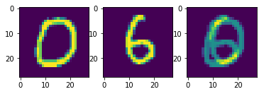
Out-of-distribution MNIST sample (source)
Which class would the third image belong to? The network could produce a distribution indicating equal confidence that the picture belongs to both classes “0” and “6”. However, in a typical classification task, we expect the neural network to be confident in only one class per image instance.
A similar phenomenon can be observed when rotating an image of the digit “1”. For rotation angles between approximately 60 and 130 degrees, the model fails to recognize the digit correctly and instead classifies it as either a “5” or a “7”, depending on the specific angle.
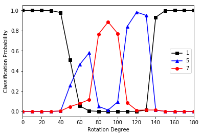
Out-of-distribution MNIST sample (source)
Both examples show that we need some form of quantification for uncertainty. This, however, is not a trivial problem. For instance, one might be tempted to introduce an additional $(K+1)$-th class to represent “uncertainty”, but such an approach assumes the existence of labeled data for the uncertain category in the first place.
This is where Evidential Deep Learning [1] comes in. Instead of modeling single point-estimate probability, the NN now acts as a sensor gathering evidence. In the above cases, instead of spitting out a uniform categorical distribution (blind guess), we encourage the network to output “I’m not sure, I see no evidence”.
Under this paradigm, the network is incentivized to assign low evidence value to non-label classes, which, assuming clean training data, lack sufficient supporting features in the input image. As a result, it prevents the model from making blind guesses when actual out-of-distribution samples appear during inference, which do not have sufficient supporting features for all learned classes.
The original paper is quite insightful, but I found the bar to be too high for readers unfamiliar with all the mathematical concepts. While we still aim to maintain a balance with the mathematical details, this post is intended to provide a higher-level view of the method and to begin from a starting point we are all familiar with: building an image classifier.
Beyond softmax
Let us formulate our problem again. Suppose that we are building a classifier to assign a class $k=1..K$ to an image $\mathbf{x}_i$. After going through a backbone network (could be anything — FNN, CNN, or ViT), the network outputs the logit vector for the instance:
Typically, we would apply a softmax activation to the logits to obtain the normalized confidence for each class:
$$ {\mathbf{p}}_i=\mathrm{Softmax}(\mathbf a_i) $$
However, this brings us back to the situation described earlier: the network is forced to select a “winner” class, even when it has no understanding of the input.
Evidential Deep Learning (EDL) offers a different perspective on this problem. Instead of modeling a “point-estimate” (in this case, a “point” is a single probability vector $\hat{\mathbf{p}}_i$) for the class distribution, EDL models a probability distribution over all possible probability vectors. Specifically, it uses the Dirichlet distribution $\mathrm{D}(\hat{\mathbf p_i} | \mathbf{\alpha}_i)$ to model the density of likely class probabilities. This is a second-order distribution: a distribution over different possible $\mathbf p$ vectors, which in turn are the good ol’ distributions over the classes.
The mathematical details are indeed scary and can be spared for later. But roughly speaking, we modify the network to output an evidence vector $\mathbf{e}_i \in [0, \infty)$ akin to a rectified logit activation. From this evidence, we derive not only the class probabilities but also a separate quantifier of uncertainty $0 < u < 1$.
The expectation for this new architecture/paradigm is intuitive:
- Knowledgeable behavior: it should behave similarly to softmax when it’s confident. When the network “successfully” predicts a correct example, the evidence $e_{ik}$ is strong at $k=\mathrm{argmax}(\mathbf y_i)$, and weak everywhere else. At the same time, the uncertainty term $u_i$ should also be low.
- Ignorant behavior: this is where EDL diverges from softmax. Consider the situation where the network is clueless. A softmax network might produce a uniform output $\mathbf p = [0.33, 0.33, 0.33]$. In contrast, a network trained with evidential objectives expresses ignorance by shrinking total evidence toward zero when it cannot correctly explain a sample: $\mathbf{e} = [0, 0, 0]$ (which corresponds to “I see no evidence”). This state mathematically pushes the uncertainty term toward its maximum value $u=1.0$ (corresponding to “I’m not sure”).
In light of this, EDL treats the neural network as a sensor that collects evidence to form a “subjective opinion”. Modeling evidence instead of probability directly enables us to:
- Explicitly quantify epistemic uncertainty (confusion between known classes, e.g., a handwritten ‘1’ that looks like a ‘7’)
- Reflect aleatoric uncertainty (total lack of knowledge, e.g., the cat image) through class-level belief distributions.
A natural question arises: how would this be implemented as an actual learning task?
The construct of Evidential Learning
Since the essence of any learning task is determined by its loss function, it is natural to address this early on. The objective for evidential learning is a compound loss of a risk term and a regularization term:
${\mathbf p}_i$ and $\tilde\alpha_i$ will be introduced later. The first term $\mathcal{L}^{err}$ acts similarly to the standard cross-entropy or mean squared error loss we are used to. The second term is a Kullback-Leibler (KL) divergence penalty. While we will dissect the terms later, the “magic” of the zero-evidence output comes almost entirely from the regularization term.
To understand how this works, let’s go back to the step where the network generates the logits $\mathbf{a} \in \mathbb{R}^K$ and continue the forward pass.
To convert these into evidence, we first apply a non-negative activation function (ReLU or exp):
$$ \mathbf{e}_i=\mathrm{ReLU}(\mathbf a_i) $$
In the theory of Subjective Logic, evidence determines the parameters for a Dirichlet distribution, which is simply:
$$ \alpha_{ik} = e_{ik} + 1 $$
We then calculate the Dirichlet strength $S_i$, which is simply the sum of all parameters:
$$ S_i=\sum_{k=1}^K \alpha_{ik} $$
The strength quantifies the magnitude of belief across all classes. From these quantities, we can extract the expected class probability for decision-making:
Next, we can compute the vector $\tilde\alpha_i$ as a function of $\alpha_i$ (introduced later), and now we have enough terms to calculate the loss $\mathcal L_{total}$ for backprop.
The uncertainty term $u_i = K/S_i$ is not optimized directly.
Note that at the moment, it appears we are adding extra steps just to obtain a normalized score $\hat p_{ik}$ from an activation function. The real guts, however, lie in the loss terms. But now there’s too much new math! To understand what the hell is going on, we should take a step back for a moment. Spend some time internalizing how the loss function could be computed from the logits $\mathbf a_i$ before continuing.
The essence of Evidential Learning
In this section, we’ll explore the meaning behind each mathematical component and begin breaking down the new concepts we’ve encountered so far. We will eventually show how the loss function is computed, which leads to the behaviors we discussed in Section 1.
Quantifying ignorance
Let’s build intuition for the scalar values $S_i$ and $u_i$. Recall that $\alpha_{ik}=e_{ik}+1$. The Dirichlet strength is just the sum of these parameters, quantifying the total mass of opinions the network has formed about its input data. This is directly linked to the uncertainty term, which governs the two behaviors we derived earlier:
- The “I don’t know” case: If the network sees no meaningful evidence in the input ($e_{ik} \approx 0$ for all $k$), then every parameter $\alpha_{ik} \approx 1$, which leads to $S_i \approx \sum_{k=1}^K1=K$. Hence:
$$ u_i \approx \frac{K}{K}=1.0, $$
which is the mathematical definition of maximum epistemic uncertainty.
- The “confident” case: Recall that $S_i=\sum_k (e_{ik}+1)$. As the network learns to gather evidence for a class (e.g., learning the features to classify a ‘7’ in MNIST), the corresponding $e_{ik}$ grows. As $S_i \to \infty$, $u_i \to 0$.
So, in a well-trained evidential network, $S_i$ acts as a proxy of accumulated evidence. If it is large, the network is knowledgeable; otherwise, it is ignorant.
How is no-evidence modeled?
The first point in the previous section relies on a property:
How do we force the network to output zero evidence when it is confused? Standard neural networks have no incentive to do this. Remember that the standard cross-entropy loss is:
which restricts the update of the neural network’s weights to depend solely on the confidence of the correct class. This objective also allows the model to output arbitrary probabilities for other classes without penalty. They are forced to distribute probability mass across known classes.
In EDL, we encourage the evidence assigned to non-label classes to remain low during training by regularizing the predictive distribution toward the uniform Dirichlet distribution $D(\cdot | \mathbf 1)$, a state of complete ignorance, where the parameters are $\alpha_{ik}=1 \Leftrightarrow e_{ik} = 0$.
This regularization pushes the model toward a state of ignorance unless it has clear evidence from the data to support a specific class.
$$ R({\mathbf p}_i, \tilde\alpha_i) = KL[D(\mathbf p_i|\tilde\alpha_i)\ ||\ D(\mathbf p_i|\mathbf 1)] $$
Details about the Dirichlet distributions can be found later. For now, we understand that $D(\mathbf p_i|\tilde\alpha_i)$ corresponds to the network’s output.
Evidence masking ($\tilde\alpha_i$)
But the network cannot learn anything if we keep pulling all evidence towards zero. We need a mechanism to punish evidence for the wrong classes while letting evidence for the correct class grow freely.
We construct a modified parameter vector $\tilde{\alpha}_i$ by masking out the correct class parameters from the original $\alpha_i$:
Let understand this with a concrete example. Suppose we have a 3-class problem. The ground truth is Class 0 ($\mathbf y = [1, 0, 0]$).
- Prediction: the network outputs evidence that results in parameters $\alpha_i = [10, 4.5, 2.6]$
- Mask: for the correct index, we ignore the network’s output and replace it with $1$. For non-label classes, we keep the network’s output. We would get $\tilde\alpha_i = [1, 4.6, 2.6]$.
The KL term then calculates the between the distribution defined by $\tilde\alpha_i$ w.r.t. the uniform distribution (where $\alpha = \mathbf{1}$). This pulls the $\tilde\alpha_{ik}$ for non-label classes to 1, which pulls the corresponding evidence values towards zero. The evidence of the true label is unaffected by regularization.
The network is now incentivized to drive the evidence of non-label classes toward zero, which, assuming clean training data, lack sufficient supporting features in the input image data. As a result, it reduces blind guesses when actual out-of-distribution samples appear during inference, which do not have sufficient supporting features for all learned classes.
Up to now, we have addressed the following questions:
- How uncertainty $u_i$ is quantified through evidence
- How is evidence reduced to zero when there is no supporting feature in the input data
The loss function
We conclude by examining the loss function after defining all the important details. Recall that the loss is a compound loss:
As previously discussed, the purpose of the regularization term is to pull the evidence for non-label classes to zero while leaving out the evidence for the ground-truth class. This target class evidence is optimized through the risk term:
This is elegant because it decomposes the objective into two clear goals:
- Prediction error: the standard sum of squared errors (SSE) between the one-hot label and the predicted probability distribution. Note that we compute the loss over all classes, not just the target class.
- Variance: The second term reflects the variance of the Dirichlet distribution. As the confidence increases, the predictive variance will shrink.
Regularization annealing
$$ \lambda_t = \min\left(1.0, \frac{t}{10}\right) $$
This starts the regularization at $0$ and linearly increases it to $1.0$ over the first 10 epochs, which allows the network to learn initial patterns before being heavily penalized for misassigned evidence.
Implementation
The implementation becomes elegant and straightforward once we have worked through all the theoretical details.
- Start with a backbone architecture.
- Head modification: Replace the final Softmax layer with a ReLU (or similar non-negative) activation to ensure positive evidence $\mathbf e_i$
- Forward pass: compute $\alpha_i = \mathbf e_i + 1$ and $S = \sum_{k}\alpha_{ik}$
- Inference: the probability for each class is calculated as $\mathbf p_i = \alpha_i/S_i$, and the uncertainty is $u_i = K/S_i$
- Backprop: calculate the custom loss function; annealed over epochs to prevent early convergence to the uniform distribution
The official implementation for the paper could be found here.
Appendix I: The Dirichlet distribution
(Coming soon)
References
[1] Murat Sensoy, Lance Kaplan, and Melih Kandemir. 2018. Evidential deep learning to quantify classification uncertainty. In Proceedings of the 32nd International Conference on Neural Information Processing Systems (NIPS'18). Curran Associates Inc., Red Hook, NY, USA, 3183–3193.
Acknowledgement
This post represents my interpretation of the concept and may not be entirely correct. Some parts were cross-checked with the original material using ChatGPT and Gemini Pro.